Hierarchy of Big Men From the 2018 NBA Draft: Part Two

Analyzing all the big men taken in the 2018 draft using a blend of statistics, self-created models, and observations. Part two incorporates self-created model to predict future success of these players.

Part one allowed us to differentiate the big men of the 2018 draft by using their college stats to asses their skill sets; part two takes a more sophisticated approach. To predict success at the next level I formulated a multitude of models that take different statistics and measurements to compute an overall draft score. Let's take a look at two of the best models:

Model One

To create a model that predicts future success of these prospects I first had to compile a data set of statistics and measurements of current NBA players. My data set included every NBA player aged 24 to 32 (who also was drafted between 2005 and 2014) that played a significant amount of minutes during the 2017-2018 season (significance determined by John Hollinger in his PER rankings on ESPN.com). For the purposes of these models we are predicting how successful players will be in their primes, and therefore, the only players included in the data set are ones who are in their primes (I theorized that on average the best range for players in their prime are the parameters I set, as it gives players enough time to get adjusted to the play of the league, while also not accumulating too much mileage). To produce a model score, I used Hollinger's PER as my dependent variable (Hollinger's PER has been one of, if not the most, comprehensive and accurate statistic in conveying the impactful an NBA player has on their team). For the first model I used True Shooting Percentage, Points Per Minute, Defensive Win Shares, and the difference between a player's height and their wingspan as my independent variables (statistics compiled from their college averages, measurements taken from their combine results). In order to produce accurate results that followed the classical linear model assumptions, I had to transform my dependent variable by cubing it (as the plot of my residuals followed a pattern that resembled a cubed function). After transforming my dependent variable, I was able to produce the following ranking of the 2018 draft class by using the predict function in R. The scores shown below are the cubed values of their predicted PER. The reason I didn't convert the cubed value back to its PER form is due to the misleading nature of the PER predicted value. Due to issues with heteroskedasticity, the PER value produced is skewed, and thus, is not an accurate prediction for PER (the issue with heteroskedasticity is a result of much higher variance for players who excelled in college to those who did not do well in college). However, I can still use the scores produced as a value to rank the player's by; players with higher scores are still projected to perform better in the league (all their scores are skewed, therefore, if a player has a higher score than another player, even without issues with heteroskedasticity the player would still have a higher score). Here are the scores (only the scores of big men shown below):

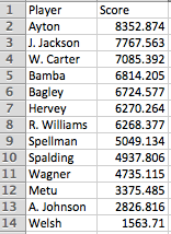
The top five bigs selected in the draft have the five highest scores (a good sign for the accuracy of the model). Ayton dominates the competition with a staggering score of 8352.874 (staggering compared to the competition), followed by Jaren Jackson who also has a relatively high score of 7767.536. Jackson and Ayton both project well in this model as they blend great length with efficient scoring. Wendell Carter and Mo Bamba (perhaps the two players who fared the best in part one of this analysis), also perform well in this model, as they rank third and fourth in a very deep big man class. Bagley falters a bit in this model (being the #2 pick overall), due to a lack of size and defensive ability, both of which are legitimate hinderances to Bagley's chances of becoming an all star big in the league. The player who sees the most value from this model is Kevin Hervey. Hervey, the #57 pick overall and the second to last big man drafted, finishes sixth in this model. Hervey displayed efficient shooting in college, but what really adds value to his score is his ridiculous 7'4 wingspan at only 6'8. The model adds evidence to Hervey's case of becoming a solid player at the next level, while also simultaneously removing a lot of the uncertainty of his game translating due to playing in a smaller conference.

Model Two

Like model one, model two uses PER as a dependent variable to produce a draft score. However, instead of using the full data set that model one used, it uses an abbreviated version of the data set that only incorporates big men. By doing this, I can isolate variables that better predict the success of big men compared to guards and wings (i.e. block rate), while also eliminating unfair competition (i.e. stacking big man against guards in stats like usage rate; the rate in which a player is used in the offense). This model uses the two aforementioned stats (blocks and usage rate), as well as true shooting percentage as its independent variables. Once again heteroskedasticity is an issue, so the draft score is not reflective of what their predicted PER will be, it is a simply a value that allows us to rank them against other prospects. Here are the scores:

From the model, block rate has the strongest correlation with PER, and it shows in the results; Jaren Jackson, Mo Bamba, and Robert Williams, all long rim-protecting bigs, place in the top three for scores. Jaren Jackson absolutely dominates in this model with a score of 25.08901, mostly due to an unworldly 14.3 block rate in college. If anything, this model illustrates that the players whose games will translate the most fluidly to the next level are dominant shot blockers, or as discussed in part one, lengthly rim protecting/rim running bigs. Ayton who ranked first in the first model, falls to fourth due to his relatively subpar block rate in college (6.1). Ayton's inability to protect the rim is his one real weakness, and is the reason other players like Jackson and Bamba may be more of a guarantee to be successful at the next level. Bagley once again falters in this model, as he lacked any presence at the rim in college (2.6 block rate); adding evidence to the fact that Bagley's weaknesses will hold him back in the NBA.

Overall, the second model tends to favor rim protecting bigs (Bamba, Wiliams, Metu), while the first model favors versatile bigs (Hervey). Players who qualify as versatile and rim protecting bigs fared well in both models (Carter, Ayton, Jackson). The models add evidence to back the theory from part one: players that fit into one of the big men categories (versatile or rim protecting), are more likely to succeed in the NBA, while also adding to the theory by suggesting that players who fit into both categories have the best chance of succeeding. However, it appears rim protecting bigs have a better chance than versatile bigs to be successful at the next level, due to the high correlation between block rate and PER.

Part three will wrap up this analysis of the big man draft class by creating a definitive hierarchical ranking that encompasses everything discussed in the first two parts.